
Computer Applications I :: Lessons :: The VLookup Function
The VLookup Function
The VLookup Function stands for vertical lookup and is similar to the Choose Function, but it allows you to display data based on a range of numbers instead of just a single number.
- Create your spreadsheet like the one below:
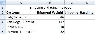
We will use the VLookup Function to display the shipping and handling costs based on the weight. In order to use the VLookup Function we need to create a table array that contains the ranges of numbers that will determine the cost.
- Click in Cell A8.
- Create the table array below:
| Weight | Shipping |
|---|---|
| 0 - 10 | 6.49 |
| 21 - 30 | 8.73 |
| 31 - 75 | 12.56 |
| 76 - Over | 25.00 |
- Convert the shipping costs to Currency Style.
- Click in Cell C3.
- Type "=VLOOKUP(B3, $A$9:$B$12, 2)".
The VLookup Function lookup value or search key is the cell in your main table that determines the value the VLookup Function will look up. The second parameter of the function is the location of the table array. You can type this in or click-and-drag to add it to the function. Notice that the cell references are locked so we can easily copy this formula to other cells. Finally, the column index number indicates how many columns are in the table array. In this course we will always use 2-column table arrays so you can just remember to always use 2 for this parameter.
After entering the formula you may have noticed that you get an error message in the cell. This is because there is an error in our table array. The VLookup Function can determine the ranges on its own and we only need to provide the lowest number for each range.
- Change the table array so it contains the lowest number in each range.
- Use the Fill Handle to drag the formula in Cell C3 to Cell C6.
- Create a new table array based on the information below:
| Weight | Handling |
|---|---|
| 0 - 5.5 | 3 |
| 5.6 - 20 | 12 |
| 21 - 50 | 48 |
| 51 - Over | 154 |
- Convert the handling costs to Currency Style.
- Use the VLookup Function to determine the handling costs.
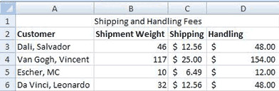
Remember that the table array should not contain ranges of numbers since the VLookup Function will determine the ranges on its own. Your spreadsheet should look like the one below when you are done.
Sorting Data
A commom task in a spreadsheet is sorting data. You can sort by almost any type of data in Excel and Google Sheets.
Excel Instructions
- Select Cell A2 through Cell D6.
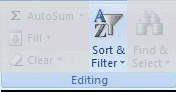
- Go to Home>Editing>Sort & Filter>Custom Sort...
Google Sheets Instructions
- Select Cell A2 through Cell D6.
- Go to the Data menu.
- Choose to sort the range by column A, A->Z.
It is important to select all of the data in your table. If you just select the items to sort the rest of the data will not move. Luckily, Excel gives you a warning if you try to do this. Once the Custom Sort window is open you can choose what field you want to sort by. Since we selected the column titles they appear in the Sort By section. If we hadn't selected the titles it would simply say "Column A" instead of "Customer." You can also choose whether to sort in ascending or descending order.
Excel Instructions
- Sort the table by "Shipment Weight" in Ascending Order.


