Computer Applications I :: Lessons :: The Choose Function
The Choose Function
The Choose Function allows you to automatically fill in a row or column with data based on the numeric value of another row or column. This is another time-saving function in Excel and Google Sheets and could be used for such things as converting a number 1-12 to a month of the year.
- Create your spreadsheet like the one below:
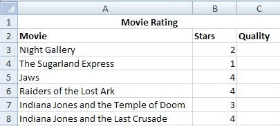
We will use the Choose Function to display the quality of a movie based on its star rating.
- Click in Cell C3.
- Type "=CHOOSE(B3, "Poor", "Fair", "Good", "Excellent")"
- Use the Fill Handle to drag the formula from Cell C3 down to Cell C8
Formula AutoComplete
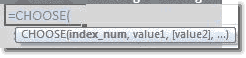
You may notice that a small window appears after you type the equal sign in Excel or Google Sheets. This window contains all of the functions included in the program and is known as Formula AutoComplete. The list will narrow down based upon what you type. If you press the "Tab" key while a function is selected that function will be entered into the cell. This is another time-saving feature that you may use. Formula AutoComplete is also important for showing you the required parameters of a function. After you select a function, the window will display what the function does, as well as names for the different parameters. A parameter that is required will appear normally. An optional parameter will appear in brackets, such as [value2] in the choose function example.
The index, or index_num, is the number that the choose function looks at to determine the value it will display. The values must be typed in numerical order so value 1 will correspond to the number 1 or the item after the index number. In our formula above index 1 would be "Poor", index 2 would be "Fair," and so on. The value can be text or a number, but if it is text it must be displayed inside quotes.
Now we will create a column to display the ticket price for the movies. The ticket price will again be based on the star rating.
- Type "Price" in Cell D2.
- In Cell D3 type "=CHOOSE(B3, 2, 3, 5, 8)".
- Convert the result to Currency Style.
- Use the Fill Handle to drag the formula from Cell D3 down to Cell D8.
Finally, we will create a column to display the number of showings of each movie based on the star rating.
- Type "Showings" in Cell E2
- Use the Choose Function to create a formula based on the table below
| Star Rating | Showings |
|---|---|
| 1 | 4 |
| 2 | 8 |
| 3 | 20 |
| 4 | 40 |
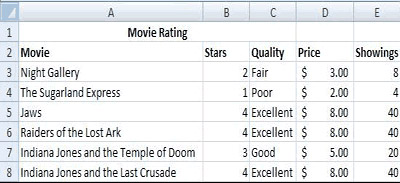
After completing the choose function your spreadsheet should look like the one below.
Line Charts
Line charts are generally used to display two or more sets of similar data. Let's create a different set of star ratings that we can use for a line chart.
- Type "New Star Rating" in Cell F2.
- Type "3," "1," "4," "4," "3," and "3" in Cells F3 through F8.
Since line charts are usually created from two sets of data you will need to select both sets of data before creating the chart.
Excel Instructions
- Highlight Cells A3 through B8.
- Hold down "Ctrl".
- Highlight Cells F3 through F8.
- Go to Insert>Charts>Line
- Give the chart the title "Star Ratings".
Google Sheets Instructions
- Highlight Cells A3 through B8.
- Hold down "Ctrl".
- Highlight Cells F3 through F8.
- Click on the Insert Chart button and select a Line Chart.
- Give the chart the title "Star Ratings".
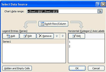
In Excel, you will notice that the legend in our chart is not labeled. We can use Select Data to fix this although it works slightly differently than labeling the axis.
Excel Instructions
- Right-click on the line chart.
- Choose Select Data....
- Click on Series1 and click "Edit".
- Type "Original Star Rating".
- Hit "OK".
- Click on Series2 and click "Edit".
- Type "New Star Rating".
- Hit "OK".