
Computer Applications I :: Lessons :: Spreadsheet Basics
Terms to Know
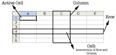
- Column - Columns are oriented vertically in spreadsheets, and are named by uppercase letters in Excel and Google Sheets.
- Row - Rows are oriented horizontally in spreadsheets, and are named by numbers in Excel and Google Sheets.
- Cell - A cell is the intersection of a row and a column, and is named by the combination of the column name followed by the row name. For example, Cell C3 would be in column C and row 3.
- Active Cell - This is the currently-selected cell. It is highlighted with a black box in Excel and a blue box in Google Sheets.
Spreadsheet Titles
It is important to give your spreadsheets titles. You may not be the only person looking at these numbers so giving the spreadsheet a title another person will better understand what the data is supposed to show. It is also important to give headings to rows and columns so it is easy to see what that data represents.
- Click in Cell A1
- Type "Apple Daily Sales"
You will notice after typing the spreadsheet title that it does not fit in the cell. This will happen often, but there are many ways to resize a column or row so the data will fit.
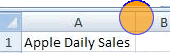
- Move your mouse to the line circled
- Click-and-hold the line to drag it right
- Adjust the line to just fit the text
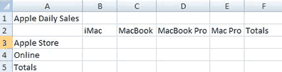
Now we must set up the column and row headings so that all the numbers we enter into the spreadsheet make sense.
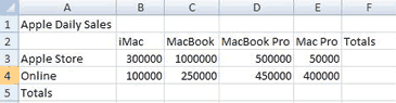
- Set up your spreadsheet like the one shown below:
- Highlight cells B2 through F2 in Excel, or columns B through F in Google Sheets. We are going to adjust the size of all these columns at once, but there are slightly different methods of doing this in Excel and Google Sheets.
AutoFit
Make sure you still have cells B2 through F2 selected in Excel, or columns B through F in Google Sheets.
Excel Instructions
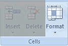
- Make sure the Ribbon is currently on the Home Tab
- Go to Home>Cells>Format>AutoFit Column Width
Google Sheets Instructions
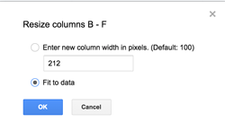
- Right-click anywhere on the selected columns and choose Resize Columns B-F
- Choose "Fit to data" and hit OK
The columns that were highlighted should now be big enough for all the words you typed.
Currency Style
Now we need to enter some data in our spreadsheet. We will also learn how to format that data correctly.
- Enter the following numbers into your spreadsheet:
You may find that some of your numbers disappear after you type them and are replaced by a number of pound signs (#####). This is because the numbers do not fit in the cell so it needs to be resized.
- Double-click on the line in between two columns to AutoFit the column to the left
Since this spreadsheet represents the amount of money made on each of the different computer models we want to add a dollar sign and two decimal places so it is obvious we are dealing with money. You do NOT want to add the dollar signs manually since this will change the data type from Number to Text and it will be more difficult to do calculations on the data.
- Highlight cells B3 through E4, which are the cells with the numbers
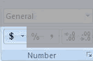
- In Excel, go to Home>Number and press the button with the dollar sign. In Google Sheets, press the dollar sign button under the menu.
The Accounting Number Format button allows you to set the currency style. Since we won't be working with currencies other than the U.S. Dollar you won't have to use the pull-down to change the format. Simply pressing the dollar sign when you have the numbers selected will set them all to currency style. Make sure you always set numbers to currency style if they involve money.
The Sum Function
Now we need to get the totals for all the rows and columns. You could do this by hand, but spreadsheets are built to do calculations so we may as well use the tool we have in front of us. The command we are going to use is known as the sum function.
Excel Instructions
- Highlight cells B3 through F3
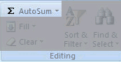
- Go to Home>Editing>AutoSum
- Repeat this process for the remaining rows and columns
Google Sheets Instructions
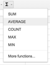
- Click in cell F3
- Click on the function button on the right side of the button bar and choose SUM
- Highlight cells B3 through E3 and repeat this process for the remaining rows and columns
Formatting the Spreadsheet
Finally, we don't want our spreadsheet to remain the boring original colors. Excel and Google Sheets include many more options to make your spreadsheet stand out. We will start by styling the spreadsheet title.
- Highlight cells A1 through F2
- In Excel, go to Home>Alignment>Merge & Center. In Google Sheets, click the Merge Cells buttons and then the Center Alignment button next to it.
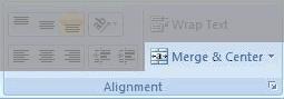
Merge & Center takes all the selected cells and merges them into one big cell. It also centers the contents of the cell. You will use this often with spreadsheet titles.
Excel Instructions
Google Sheets does not have a Cell Styles feature like Microsoft Excel. To style the cells of a Google Sheet you will have to change the background color, font, and font color manually along with the cell borders.
- Highlight Cell A1, which is the large cell you just created
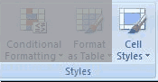
- Go to Home>Styles>Cell Styles
- Choose a style for your spreadsheet title
- Add styles to the rest of your spreadsheet
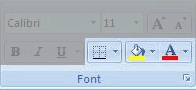
Cell styles are a quick and easy way to make your spreadsheet look nice. Alternatively, you could use the Fill Color, Font Color, and Border buttons under Home>Font to tweak the colors and styles yourself.
Creating a Bar Chart
Data on its own can be tough to read, but the addition of a chart or graph can make the data much easier to understand. Charts are simple to create in Excel and Google Sheets, but can display data in any number of ways. It is much easier to create a chart if you select the data you are going to graph first. This may not always be possible, but you should try to select the data first as often as you can.
Excel Instructions
- Highlight cells A2 through E4 and make sure the Insert Tab is selected
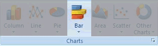
- Choose Insert>Charts>Bar
- Select one of the bar charts in the left-most column
Google Sheets Instructions
- Highlight cells A1 through E4
- Click on the Chart button on the right side of the button bar
- Select the bar chart on the left side
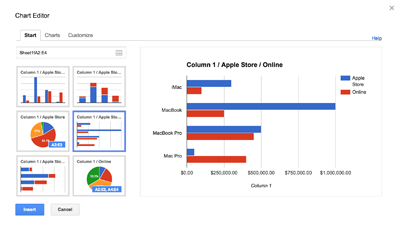
Your bar chart will be added to your spreadsheet. You can move it by clicking-and-dragging it. Bbecause we highlighted the text as well as the numbers before we created our chart some of the chart has been filled in for us. We can edit the chart to fill in the remaining data.
Editing a Chart
While Excel and Google Sheets do a fairly good job of creating your chart for you, there may be more you want to add to the chart. Additionally, you may want to change the look of the chart.
Excel Instructions
When your chart is selected you will notice three new tabs appear to the right of the other tabs. These tabs will be under a heading that says Chart Tools.
- Click on your chart to select it
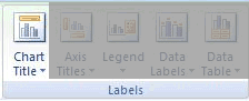
- Select the Layout Tab under Chart Tools
- Go to Layout>Labels>Chart Title
- Choose a Centered Overlay Title
- Type "Apple Daily Sales" for the title
Google Sheets Instructions
- Click on the title of your chart and change it to "Apple Daily Sales"
- Right click to add titles to the horizontal and vertical axes
You can also change the size, color, and style of text in the chart. Right-clicking on anything in the chart will allow you to change its properties.
- Change the style of the chart title so it stands out
- Change the font of the remaining text
- Change the font size of the remaining text to 14.
- If any text is overlapping pull on the edges of the chart to make it bigger
It is important that you make sure the chart looks neat and there isn't any overlapping text. If text does end up overlapping you can either increase the size of the chart or decrease the size of the font.


